Powersort

Introduction

Powersort is a modern sorting algorithm (proposed 2018 in Nearly-Optimal Mergesorts: Fast, Practical Sorting Methods That Optimally Adapt to Existing Runs) that keeps the worst-case guarantees of Mergesort, and works faster on "easy" inputs. This leads us to first define what is meant by easy and hard, and how we can exploit these ideas reliably without spending much additional computation on them.

Even though all the following can be applied to any comparable type of object (e.g. strings), we use integers for easy visualization. Consistent with C-style languages, we write the array as $A = (a_0, a_1, \dots, a_{n-1})$ for length $n \in \mathbb{N}$, where $a_i$ denotes the element at index $i$. First off, we consider the arguably "easiest" input possible for sorting; an ascending array, so an array that is already sorted. In this case, nothing needs to be done:

Next up, let's think about hard inputs. A very straightforward initial idea could be just taking the opposite of the previous array; one that is fully descending:

However, this should not be considered hard: we can simply reverse the array in linear time without any comparisons.

A harder input looks like the following (though there are many other valid examples). The bars can be swapped by drag-and-drop, so try out other arrangements to get more familiar.

A way to quantify why this one is harder than the previous inputs is counting the contiguous sections that are already monotone. For indices $0 \le i \le j < n$, we write $A[i..j] = (a_i, a_{i+1}, \dots, a_{j-1}, a_j)$ for the contiguous section of $A$ from position $i$ to $j$. From now on, these monotone sections will be called runs.

More precisely, an ascending run of $A$ is a section $A[i..j]$ with $0 \le i \le j < n$ such that $a_i \le a_{i+1} \le \dots \le a_j$ and that $j$ is maximal, i.e. it can't be increased without breaking the monotonicity of the elements. A descending run is defined analogously. In this article, we use the word run for both ascending and descending runs. The runs are color-coded in the figures so that two neighboring runs have different colors. We can now state more precisely that the arrays shown at the start of the post each consist of a single run, while this new hard input decomposes into several shorter runs.

The measure we use to describe hardness of inputs is entropy. Usually in information theory, it is used to measure the amount of "surprise" a random variable (RV) has, so how much information is revealed by seeing the realization of the RV. The commonality with runs for adaptive sorting is that in both cases, some whole object taking up 100%, be it the entire array or the probability mass of a RV, is split up into parts that partition it. If a RV has a lot of information, it will be split up into many small parts, and if it has little information, it will be split up into fewer parts. In the limit, just having one possible outcome with 100% chance has entropy of 0, and the same applies here if there is only one run, either ascending or descending. We won't use more details on entropy going forward, so we skip a formal derivation.

Merging of runs

To use these runs productively for sorting, we can borrow the merge-operation of the Mergesort algorithm. It takes two runs that are next to each other and merges them to one run that contains all the elements of the two input runs. The merge works by maintaining two pointers, one for each run, and repeatedly picking the smaller element. Since both runs are already sorted, this produces a sorted result in linear time:

void merge(int *arr, int left, int mid, int right, int *buf) {
    int i = left, j = mid, k = 0;
    while (i < mid && j < right)
        buf[k++] = (arr[i] <= arr[j]) ? arr[i++] : arr[j++]; // choose smaller element
    while (i < mid) buf[k++] = arr[i++]; // clear left run
    while (j < right) buf[k++] = arr[j++]; // clear right run

    for (int x = 0; x < k; x++) arr[left + x] = buf[x]; // copy elements from buffer
}

For more details on optimizing merge operations, see section B.1 Merging of Nearly-Optimal Mergesorts.

The cost of merging two runs is proportional to their combined length, as each element is compared and copied exactly once: $\text{len}(R_i) + \text{len}(R_j)$.

Let $k$ be the number of runs at the very start, then exactly $k-1$ merge-operations are needed to sort the whole array, as each time the number of runs is reduced by 1, and the sorted array is known to be just one big run.

Finding good merge trees

So far, it is not specified in which order which runs are supposed to be merged. Experimenting with the array above shows that any order of merges results in a correctly sorted array. The difference lies in that different merge-orders generally take a different amount of time.

Let's consider the array below, in which this effect is particularly nice to see:

There are 3 runs, the left one being by far the longest with 7 items, and the middle and right one shorter with size 2 and 1 respectively. Before reading further, try walking through both choices for the first merge-operation by hand.

The two possible merge orders are explained below:

$R_1$ (len 7)

$R_2$ (len 2)

$R_3$ (len 1)

$R_1+R_2$ (len 9)

Sorted (len 10)

Total Cost: $(\text{len}(R_1) + \text{len}(R_2)) \; + \; (\text{len}(R_1+R_2) + \text{len}(R_3)) \; = \; (7 + 2) + (9 + 1) = 9 + 10 = 19$

This merge order is inefficient, as it creates an "unbalanced" order of operations. The intermediate array $R_1+R_2$ seems unnecessarily big.

$R_1$ (len 7)

$R_2$ (len 2)

$R_3$ (len 1)

$R_2+R_3$ (len 3)

Sorted (len 10)

Total Cost: $(\text{len}(R_2) + \text{len}(R_3)) \; + \; (\text{len}(R_1) + \text{len}(R_2+R_3)) \; = \; (2 + 1) + (7 + 3) \; = \; 3 + 10 = 13$

Merging the two smaller runs $R_2$ and $R_3$ first is much less expensive, as the intermediate array they create is much shorter than when using the array $R_1$.

Related example: Matrix Chain Multiplication

A similar idea appears in a different application: matrix multiplication. When multiplying three matrices $A \times B \times C$, the result is identical whether we compute $(A \times B) \times C$ or $A \times (B \times C)$, as both matrix-multiplication and merging of arrays are associative. However, the computational cost can differ dramatically.

Consider three matrices with dimensions:

$A$: $10 \times 30$
$B$: $30 \times 10$
$C$: $10 \times 30$

Multiplying two matrices of dimensions $(m \times n)$ and $(n \times p)$ costs $m \cdot n \cdot p$ scalar multiplications and results in a matrix of size $m \times p$.

The difference is a factor of $3\times$, solely from choosing a different order of operations: creating large intermediate results can heavily influence overall runtime.

The Power of a Run

From the merge order examples above, we saw that first merging "similar-sized" runs leads to better performance. But checking all possible merge orders to find the optimal one would be far too expensive: there are exponentially many possible merge trees. Powersort's key insight is a simple method that produces a nearly-optimal merge order in linear time: assign each pair of consecutive runs a cheap to calculate measure called power, then always merge the pair with the highest power first.

Consider two consecutive runs $R_1$ and $R_2$, where $R_1$ starts at position $s_1$ with length $n_1$, and $R_2$ immediately follows with length $n_2$. Define their midpoints as fractions of the total array length $n$:

$$ \begin{aligned} m_1 &= \frac{s_1 + \frac{n_1}{2}}{n} \\ m_2 &= \frac{s_1 + n_1 + \frac{n_2}{2}}{n} \end{aligned} $$

Both midpoints lie in the interval $[0, 1]$. The power of the run pair is defined as the first bit position where the binary representations of $m_1$ and $m_2$ differ, i.e., the smallest integer $k \ge 1$ such that: $$\lfloor 2^k \cdot m_1 \rfloor \neq \lfloor 2^k \cdot m_2 \rfloor$$

Why does this work? Imagine recursively splitting the array in half, like building a binary search tree over positions. At each level, we ask: do the two midpoints fall into the same half, or different halves?

High power (e.g., 4 or 5): The midpoints are close together—they only diverge after many splits. These runs are "locally adjacent" and should be merged early, producing a small intermediate result.
Low power (e.g., 1 or 2): The midpoints are far apart—they diverge after just one or two splits. These runs span a large portion of the array and should be merged late, only after their smaller neighbors have been combined.

This bisection approach directly connects to merge tree structure. An optimal merge tree for balanced data recursively splits the array in half, similar to how mergesort divides its input. The power measure effectively asks: at what depth of this hypothetical binary splitting would these two runs end up in different halves? Runs that diverge late (high power) are neighbors in this conceptual tree structure and should be merged first to minimize intermediate result sizes. In our earlier example with $R_1$, $R_2$, and $R_3$, the power calculation correctly identified that $R_2$ and $R_3$ (power 3) are more "locally adjacent" than $R_1$ and $R_2$ (power 1), matching the optimal merge order we found by hand.

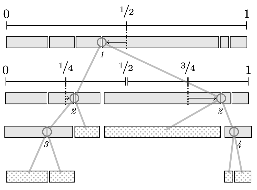
Binary partitioning tree showing from original Powersort publication — Figure from Munro & Wild, 2018 (the original Powersort publication), showing the partitioning tree for a more complex input array.
The tree recursively bisects the interval [0,1] at powers of two (1/2, 1/4, 3/4, etc.). The italic numbers show the power of each node, which determines the merge order. Higher powers (deeper in the tree) correspond to runs that are closer together and should be merged first.

Stack-Based Execution

Powersort processes runs left-to-right, maintaining a stack of pending runs. When a new run is discovered, we compute its power relative to the run on top of the stack. The crucial invariant: powers on the stack must be weakly increasing from bottom to top.

If the new run's power is smaller than some powers on the stack, those runs must be merged first (they represent "more local" pairs that should have been handled earlier). The algorithm pops and merges until the invariant is restored, then pushes the new run.

The following code comes from the NumPy implementation, slightly simplified for this post:

static int found_new_run_(type *arr, run *stack, int *stack_ptr, int n2, int n, buffer_ *buffer)
{
    if (*stack_ptr > 0) {
        int s1 = stack[*stack_ptr - 1].s;
        int n1 = stack[*stack_ptr - 1].l;
        int power = powerloop(s1, n1, n2, n);
        while (*stack_ptr > 1 && stack[*stack_ptr - 2].power > power) {
            merge_at_(arr, stack, *stack_ptr - 2, buffer);
            stack[*stack_ptr - 2].l += stack[*stack_ptr - 1].l;
            --(*stack_ptr);
        }
        stack[*stack_ptr - 1].power = power;
    }
}

The while-loop collapses the stack: as long as the second-to-top run has a power greater than the new power, it gets merged with the top run. This ensures high-power (local) merges happen before low-power (global) ones.

Computing Power Efficiently

The definition of power involves comparing binary expansions of fractions, which sounds like it might need floating-point arithmetic. The powerloop function avoids this entirely by working with integers and simulating the bit extraction process.

The powerloop function from the NumPy implementation demonstrates this:

static int powerloop(int s1, int n1, int n2, int n)
{
    int result = 0;
    int a = 2 * s1 + n1;  /* 2 * midpoint1 */
    int b = a + n1 + n2;  /* 2 * midpoint2 */
    while (true) {
        ++result;
        if (a >= n) {        /* both bits are 1 */
            a -= n;
            b -= n;
        }
        else if (b >= n) {   /* a's bit is 0, b's bit is 1 */
            break;
        }
        a <<= 1;
        b <<= 1;
    }
    return result;
}

Line-by-line explanation:

Initialization: We want to compare $m_1 = (s_1 + n_1/2) / n$ and $m_2 = (s_1 + n_1 + n_2/2) / n$. To avoid fractions, we scale everything by $2n$:

a = 2 * s1 + n1 represents $2n \cdot m_1 = 2s_1 + n_1$
b = a + n1 + n2 represents $2n \cdot m_2 = 2s_1 + 2n_1 + n_2$

The loop: Each iteration examines the next bit of $m_1$ and $m_2$. The key insight: the $k$-th bit of a fraction $x$ is $1$ iff $\lfloor 2^k x \rfloor$ is odd, which happens iff $2^k x \ge \lfloor 2^k x \rfloor + 1$ after removing previous bits. In our scaled representation, a >= n tests whether the current bit of $m_1$ is $1$.

Both bits are 1 (a >= n and implicitly b >= n since $b > a$): Subtract n from both to take away this bit, then continue to the next bit.
Bits differ (a < n but b >= n): We found the first differing bit at position result. Return immediately.
Both bits are 0 (a < n and b < n): Double both values (a <<= 1, b <<= 1) to examine the next bit.

Note that $a$'s bit being $1$ while $b$'s is $0$ cannot occur: since $R_2$ immediately follows $R_1$, the midpoint of $R_2$ is always to the right of $R_1$'s midpoint, so $m_1 < m_2$ always holds.

Worked example: Let's compute the power for the runs from our earlier merge-order example: $R_1$ (length 7), $R_2$ (length 2), $R_3$ (length 1), with total array length 10.

Power of $(R_1, R_2)$: Here $s_1 = 0$, $n_1 = 7$, $n_2 = 2$, $n = 10$.

Initialize: $a = 2 \cdot 0+7 = 7, b = 7+7+2 = 16$
Iteration 1: $a = 7 < 10 $ (bit 0), $b = 16 ≥ 10$ (bit 1) → bits differ, return 1

Power of $(R_2, R_3)$: Here $s_1 = 7$, $n_1 = 2$, $n_2 = 1$, $n = 10$.

Initialize: $a = 2·7+2 = 16$, $b = 16+2+1 = 19$
Iteration 1: $a = 16 ≥ 10$, $b = 19 ≥ 10$ → both 1, subtract and double: $a = 12$, $b = 18$
Iteration 2: $a = 12 ≥ 10$, $b = 18 ≥ 10$ → both 1, subtract and double: $a = 4$, $b = 16$
Iteration 3: $a = 4 < 10$ (bit 0), $b = 16 ≥ 10$ (bit 1) → bits differ, return 3

Since power$(R_2, R_3) = 3 > 1 = $power$(R_1, R_2)$, the algorithm merges $R_2$ and $R_3$ first. This matches the optimal order we identified earlier.

Caching Behaviour

Beyond the theoretical cost analysis, Powersort's merge order also has practical performance benefits related to modern CPU architecture. The cost analysis above counts element copies, but real-world performance also depends on cache efficiency. Modern CPUs have multiple levels of cache (L1, L2, L3) that are orders of magnitude faster than main memory. Algorithms that keep their working set small and access memory sequentially run much faster than those that have irregular accessing patterns.

// TODO: double check calculations and source. Ignore in review for now.
Consider, for example, the Intel Core™ i5-12400, a typical mid-range processor found in many home computers:

L1 Cache: 48 KB per core
L2 Cache: 7.5 MB
L3 Cache: 18 MB

If we're sorting 32-bit integers (4 bytes each), the L1 data cache can hold approximately $48.000 / 4 = 12.000$ integers per core, L2 can hold $7.500.000 / 4 \approx 2.000.000$ integers, and L3 can hold $18.000.000 / 4 \approx 4.700.000$ integers.

When merging two runs, the CPU streams through both, comparing elements and copying them to a buffer. If both runs fit in cache, this is fast. If they don't, the CPU repeatedly stalls waiting for main memory.

Powersort's "merge small neighbors first" strategy is cache-friendly for two reasons:

Small working sets: High-power merges combine short, adjacent runs. Their combined data often fits entirely in L2 or L3 cache, making the merge fast. Low-power merges (spanning large portions of the array) happen last, when there's no choice but to process more data.
Temporal locality: Runs are pushed onto the stack as they're discovered by scanning left-to-right. When two high-power runs get merged immediately, their elements were just touched, so they're likely still in cache.

In contrast, a left-to-right merge order would repeatedly stream through a growing intermediate result, evicting useful data and causing cache thrashing.

Closing thoughts

Powersort is an elegant piece of computer science because it is both effective in practice and has some neat theory behind it as well. When I first looked into the topic, I didn't find any source that introduces the core ideas of Powersort in a "semi-formal" way that is mostly self-contained.

As further material, the official publications provide detail and proofs this post does not plan to have, but for me also the public pull requests were very interesting sources to read; see for example the one for the official Python language (https://github.com/python/cpython/pull/28108).

This post also didn't really touch on the history of Powersort so far. The idea of exploiting pre-existing runs already appeared in Donald Knuth's The Art of Computer Programming, and was extended to TimSort by Tim Peters to use a heuristic merge order that is cache-friendly (compare earlier section). Later, a bug was found in TimSort where some inputs created really bad merge-orders, leading open a gap for a better merge-policy.

Powersort's theoretical guarantee distinguishes it from TimSort: while TimSort uses clever heuristics, Powersort provably achieves merge costs within $O(n)$ of the information-theoretic optimum (measured as entropy of run lengths).

The publication of Powersort is still relatively new, so there are some encouraging places left where there has not yet been an implementation (like it was for NumPy in my case).

References

Powersort Algorithm:

Munro, J. Ian, and Sebastian Wild. "Nearly-Optimal Mergesorts: Fast, Practical Sorting Methods That Optimally Adapt to Existing Runs." 26th Annual European Symposium on Algorithms (ESA 2018).
Python CPython Pull Request #28108 - Powersort implementation discussion and code
NumPy Pull Request #29208 - Powersort implementation in NumPy

Related Sorting Algorithms:

Timsort (Wikipedia) - Predecessor algorithm that inspired Powersort
Auger, Nicolas, et al. "On the Worst-Case Complexity of TimSort." ESA 2018.

Other

Matrix chain multiplication (Wikipedia) - other problem where operation order influences runtime
Locality of reference (Wikipedia) - relevant for stack-based implementation of Powersort