Powersort
Introduction
Powersort is a modern sorting algorithm (proposed 2018 in Nearly-Optimal Mergesorts: Fast, Practical Sorting Methods That Optimally Adapt to Existing Runs) that keeps the worst-case guarantees of Mergesort, but works faster on inputs that already contain useful order. This leads us to first define what we mean by easy and hard inputs, and how an algorithm can exploit that structure without spending much additional work finding it.
Even though all of these ideas can be applied to any comparable type of object (e.g. strings in lexicographical order), we use integers for convenience. Consistent with C-style languages, we write the array as \(A = (a_0, a_1, \dots, a_{n-1})\) for length \(n \in \mathbb{N}\), where \(a_i\) denotes the element at index \(i\). First off, we consider the arguably easiest input possible for sorting; an ascending array. In this case, nothing needs to be done:
Next up, let's think about hard inputs. A natural way to measure how "unsorted" an array is: the inversion count as the number of pairs \((i, j)\) with \(i < j\) but \(a_i > a_j\). The ascending array above has zero inversions, which lines up with the intuition that it's easy. The input with the most inversions is the fully descending array, with \(\binom{n}{2} = n(n-1)/2\) inversions (all subsets of size 2):
Yet we can just flip it and be done immediately. So why does the inversion count suggest this is the hardest input? Because it measures difficulty for a specific class of algorithms. Insertion sort, for example, runs in \(\Theta(n + \text{Inv}(A))\) time: each inversion corresponds to one element moving left past another element, so inputs with many inversions are harder. For algorithms of this kind, the descending array is exactly worst-case.
So whether an input is "hard" depends on which structural property the algorithm exploits. Inversion count captures pairwise disorder and is the right metric for algorithms that fix one pair at a time. But an algorithm that can detect and reverse entire sorted sections treats the descending array as trivially easy. This is the kind of structure Powersort exploits.
One such promising hard candidate for such an algorithm might look like the following: (the bars can be swapped by drag-and-drop, so try out other arrangements to get more familiar)
The runs are color-coded in the figures so that two neighboring runs have different colors. We can now state more precisely that the arrays shown at the start of the post each consist of a single run, while this new hard input decomposes into several shorter runs.
A way to quantify why this one is harder than the previous inputs is counting the contiguous sections that are already sorted. For indices \(0 \le i \le j < n\), we write \(A[i..j] = (a_i, a_{i+1}, \dots, a_j)\) for the subarray of \(A\) from position \(i\) to \(j\). From now on, if such a section is monotonic, it will be called a run.
More precisely, an ascending run of \(A\) is a section \(A[i..j]\) with \(0 \le i \le j < n\) such that \(a_i \le a_{i+1} \le \dots \le a_j\) and that \(j\) is maximal, i.e. it can't be increased without breaking monotonicity. A descending run is defined similarly, except that we require \(a_i > a_{i+1} > \dots > a_j\) to be strictly decreasing. We use the word run for both ascending and descending runs.
In the actual algorithm, a descending run is reversed immediately after it is detected. So from that point on, all pending runs are treated as ascending runs, and every later merge operates on ascending inputs only. For a brief implementation-oriented summary of how NumPy as a real world use case handles this, see the appendix.
Merging of runs
To use these runs productively for sorting, we can borrow the merge-operation of Mergesort. It takes two runs that are next to each other and merges them to one run that contains all the elements of the two input runs. Since descending runs have already been reversed at detection time, the merge routine below only needs to handle ascending runs. The merge works by maintaining two pointers, one for each run, and repeatedly picking the smaller element. Since both runs are already sorted, this produces a sorted result in linear time:
void merge(int *arr, int left, int mid, int right, int *buf) {
    int i = left, j = mid, k = 0;
    while (i < mid && j < right)
        buf[k++] = (arr[i] <= arr[j]) ? arr[i++] : arr[j++]; // choose smaller element
    while (i < mid) buf[k++] = arr[i++]; // clear left run
    while (j < right) buf[k++] = arr[j++]; // clear right run

    for (int x = 0; x < k; x++) arr[left + x] = buf[x]; // copy elements from buffer
}
(Also see section B.1 Merging of Nearly-Optimal Mergesorts)
The cost of merging two runs is proportional to their combined length, so we define the merge cost of combining runs \(R_i\) and \(R_j\) as \(\text{len}(R_i) + \text{len}(R_j)\).
Let \(k\) be the number of runs at the very start, then exactly \(k-1\) merge-operations are needed to sort the whole array, as each time the number of runs is reduced by 1, and the sorted array is known to be just one big run.
Finding good merge trees
So far, it is not specified in which order which runs are supposed to be merged. By just playing around with the array above, we can see that any order of merges results in a correctly sorted array. Technically speaking, merging runs is an associative operation. The issue is that some merge-orders need more operations/time, despite still producing the correct result. Let's consider the array below, in which this effect is particularly nice to see:
There are 3 runs, the left one being by far the longest with 7 items, and the middle and right one being shorter with size 2 and 1 respectively. Before reading further, try acting out the sorting algorithm by hand (it won't take long as there are only two choices for the merging order).
The two possible merge orders are:
Total Cost: \((\text{len}(R_1) + \text{len}(R_2)) + (\text{len}(R_1+R_2) + \text{len}(R_3)) = (7 + 2) + (9 + 1) = 19\)
A naive left-to-right merge order is very inefficient, creating an "unbalanced" order of operations. The created array \(R_1+R_2\) appears unnecessarily big. Now for the other merge order:
Total Cost: \(\text{len}(R_2) + \text{len}(R_3) + \text{len}(R_1) + \text{len}(R_2+R_3) = (2 + 1) + (7 + 3) = 3 + 10 = 13\)
Merging the two smaller runs \(R_2\) and \(R_3\) first is much cheaper. Intuitively, \(R_2\) and \(R_3\) are comparable in size, so merging them first creates only a small intermediate result. In contrast, \(R_1\) is already large, so merging it early just creates a large intermediate result that must be processed again later.
Related example: Matrix Chain Multiplication
A similar idea appears in a another important context: matrix multiplication. When multiplying three matrices \(A \times B \times C\), the result is identical whether we compute \((A \times B) \times C\) or \(A \times (B \times C)\), as both matrix multiplication and merging of runs are associative. However, the computational cost can differ dramatically.
For example, let \(A\) have size \(10 \times 30\), \(B\) size \(30 \times 10\), and \(C\) size \(10 \times 30\). Multiplying an \((m \times n)\)-matrix by an \((n \times p)\)-matrix costs \(mnp\) scalar multiplications.
The difference is a factor of 3 in this example, solely from choosing a different order of operations. A large intermediate object can heavily influence overall runtime.
Measuring difficulty: the entropy of runs
We now know that instead of only counting runs, we should look at the distribution of run lengths. Given runs \(R_1, \dots, R_k\) with lengths \(n_1, \dots, n_k\) summing to \(n\), define the run-length distribution as \(p_i=n_i/n.\) The Shannon entropy of this distribution is:
$$H = -\sum_{i=1}^{k} p_i \log_2 p_i$$This quantity, originating from information theory, is a natural measure of how difficult the merging task is. To see why, notice that every merge tree defines a weighted path length: each run \(R_i\) sits at some depth \(d_i\) in the tree, meaning its elements pass through \(d_i\) merges on the way to the root. Since each merge costs proportional to the number of elements involved, run \(R_i\) contributes \(n_i \cdot d_i\) to the total cost.
If we could merge any two runs (not just adjacent ones), minimizing \(\sum n_i \cdot d_i\) would be exactly the problem solved by Huffman coding, where symbols with probabilities \(p_i\) get codewords of length \(d_i.\) Shannon's source coding theorem then implies that the unconstrained optimum lies between \(nH\) and \(n(H+1)\).
Our setting is more constrained: only adjacent runs can be merged, so the optimal merge tree can only be at least as expensive as the unconstrained Huffman solution. This means \(nH\) is still a lower bound, but it is not generally the exact optimum once adjacency is required. The precise Powersort guarantee proved by Munro and Wild is stronger: for run lengths \(L_1, \dots, L_r\), its merge cost is at most \(H(L_1/n, \dots, L_r/n)\,n + 2n\). So Powersort is within a linear additive term of the entropy lower bound, even under the adjacency constraint.
We can validate this against the examples we already know:
- Already sorted (1 run): \(H = -(1) \log_2(1) = 0\). No merges needed, cost is \(0\). Correct.
- Maximally fragmented (\(n\) runs of length 1): \(H = -n \cdot \frac{1}{n} \log_2 \frac{1}{n} = \log_2 n\). The theorem gives a merge cost of \(n \log n + O(n)\), recovering the classic worst-case bound.
- Our 3-run example (lengths 7, 2, 1 with \(n=10\)): \(H = -\frac{7}{10}\log_2\frac{7}{10} - \frac{2}{10}\log_2\frac{2}{10} - \frac{1}{10}\log_2\frac{1}{10} \approx 1.16\). So \(nH \approx 11.6\) gives a natural lower-bound, and the better merge order from earlier with cost 13 is only slightly above it.
So the spectrum from "easy" to "hard" that we introduced at the start holds mathematically: it corresponds precisely to the entropy of the run-length distribution, which ranges from \(0\) (already sorted) to \(\log_2 n\) (no pre-existing order at all).
The Power of a Run
From the merge order examples above, we saw that first merging "similar-sized" runs leads to better performance. But checking all possible merge orders to find the optimal one would be far too expensive: there are \((n-1)!\) many possible orders to merge adjacent runs. Even if we ignore redundant sequences that result in the same operations, the number of uniquely structured merge trees still grows exponentially (following the Catalan numbers). Powersort's key insight is a simple method that produces a nearly-optimal merge order in linear time: assign each pair of consecutive runs a cheap-to-compute quantity called power. As runs are processed from left to right, these powers determine when pending runs on the stack should be merged.
Consider two consecutive runs \(R_1\) and \(R_2\), where \(R_1\) starts at position \(s_1\) with length \(n_1\), and \(R_2\) immediately follows with length \(n_2\). Define their midpoints as fractions of the total array length \(n\):
$$ \begin{aligned} m_1 &= \frac{s_1 + \frac{n_1}{2}}{n} \\ m_2 &= \frac{s_1 + n_1 + \frac{n_2}{2}}{n} \end{aligned} $$Both midpoints lie in the interval \([0, 1]\). The power of the run pair is defined as the first bit position where the binary representations of \(m_1\) and \(m_2\) differ, i.e., the smallest integer \(k \ge 1\) such that: $$\lfloor 2^k \cdot m_1 \rfloor \neq \lfloor 2^k \cdot m_2 \rfloor$$
Why is this a useful quantity? One good way to build intuition is to imagine recursively splitting the array in half. At each level, we ask: do the two midpoints fall into the same half, or different halves?
- High power (e.g., 4 or 5): The midpoints are close together—they only diverge after many splits. These runs are "locally adjacent" and should be merged early, producing a small intermediate result.
- Low power (e.g., 1 or 2): The midpoints are far apart—they diverge after just one or two splits. These runs span a large portion of the array and should be merged late, only after their smaller neighbors have been combined.
This bisection approach directly connects to merge tree structure. An optimal merge tree for balanced data recursively splits the array in half, similar to how mergesort divides its input. The power measure effectively asks: at what depth of this hypothetical binary splitting would these two runs end up in different halves? Runs that diverge late (high power) are neighbors in this conceptual tree structure and should be merged first to minimize intermediate result sizes. In our earlier example with \(R_1\), \(R_2\), and \(R_3\), the power calculation correctly identified that \(R_2\) and \(R_3\) (power 3) are more "locally adjacent" than \(R_1\) and \(R_2\) (power 1), matching the optimal merge order we found by hand.
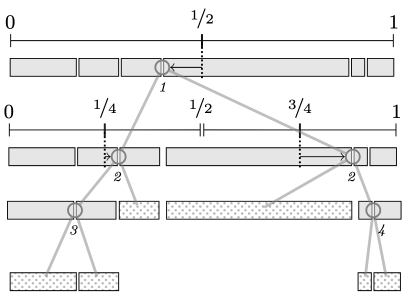
The tree recursively bisects the interval [0,1] at powers of two (1/2, 1/4, 3/4, etc.). The italic numbers show the power of each node, which determines the merge order. Higher powers (deeper in the tree) correspond to runs that are closer together and should be merged first.
Stack-Based Execution
Powersort processes runs left-to-right, maintaining a stack of pending runs. When a new run is discovered, we compute its power relative to the run on top of the stack. The crucial invariant: powers on the stack must be weakly increasing (\(\leq\)) from bottom to top.
If the new run's power is smaller than some powers on the stack, those runs must be merged first (they represent "more local" pairs that should have been handled earlier). The algorithm pops and merges until the invariant is restored, then pushes the new run.
The following code is adapted from the NumPy implementation:
static void found_new_run_(type *arr, run *stack, int *stack_ptr, int n2, int n, buffer_ *buffer)
{
    if (*stack_ptr > 0) {
        int s1 = stack[*stack_ptr - 1].s;
        int n1 = stack[*stack_ptr - 1].l;
        int power = powerloop(s1, n1, n2, n);
        while (*stack_ptr > 1 && stack[*stack_ptr - 2].power > power) {
            merge_at_(arr, stack, *stack_ptr - 2, buffer);
            stack[*stack_ptr - 2].l += stack[*stack_ptr - 1].l;
            --(*stack_ptr);
        }
        stack[*stack_ptr - 1].power = power;
    }
}
The while-loop collapses the stack: as long as the second-to-top run has a power greater than the new power, it gets merged with the top run. This ensures high-power (local) merges happen before low-power (global) ones.
Computing Power Efficiently
The definition of power involves comparing binary expansions of fractions, which sounds like it might need floating-point arithmetic. The powerloop function avoids this entirely by working with integers and simulating the bit extraction process.
The powerloop function from the NumPy implementation demonstrates this:
static int powerloop(int s1, int n1, int n2, int n)
{
    int result = 0;
    int a = 2 * s1 + n1;  /* 2 * midpoint1 */
    int b = a + n1 + n2;  /* 2 * midpoint2 */
    // note how this avoids dividing the lengths by 2 as in the original mathematical definition
    while (true) {
        ++result;
        if (a >= n) {        /* both bits are 1 */
            a -= n;
            b -= n;
        }
        else if (b >= n) {   /* a's bit is 0, b's bit is 1 */
            break;
        }
        a <<= 1;
        b <<= 1;
    }
    return result;
}
Line-by-line explanation:
Initialization: We want to compare \(m_1 = (s_1 + n_1/2) / n\) and \(m_2 = (s_1 + n_1 + n_2/2) / n\). To avoid fractions, we scale everything by \(2n\):
a = 2 * s1 + n1represents \(2n \cdot m_1 = 2s_1 + n_1\)b = a + n1 + n2represents \(2n \cdot m_2 = 2s_1 + 2n_1 + n_2\)
The loop: Each iteration examines the next bit of \(m_1\) and
\(m_2\). The key insight: the \(k\)-th bit of a fraction \(x\) is \(1\)
iff \(\lfloor 2^k x \rfloor\) is odd, which happens iff
\(2^k x \ge \lfloor 2^k x \rfloor + 1\) after removing
previous bits. In our scaled representation, a >= n tests whether the
current bit of \(m_1\) is \(1\).
-
Both bits are 1 (
a >= nand implicitlyb >= nsince \(b > a\)): Subtractnfrom both to take away this bit, then continue to the next bit. -
Bits differ (
a < nbutb >= n): We found the first differing bit at positionresult. Return immediately. -
Both bits are 0 (
a < nandb < n): Double both values (a <<= 1,b <<= 1) to examine the next bit.
Note that \(a\)'s bit being \(1\) while \(b\)'s is \(0\) cannot occur: since \(R_2\) immediately follows \(R_1\), the midpoint of \(R_2\) is always to the right of \(R_1\)'s midpoint, so \(m_1 < m_2\) always holds.
Worked example: Let's compute the power for the runs from our earlier merge-order example: \(R_1\) (length 7), \(R_2\) (length 2), \(R_3\) (length 1), with total array length 10.
Power of \((R_1, R_2)\): Here \(s_1 = 0\), \(n_1 = 7\), \(n_2 = 2\), \(n = 10\).
- Initialize: \(a = 2 \cdot 0+7 = 7, b = 7+7+2 = 16\)
- Iteration 1: \(a = 7 < 10 \) (bit 0), \(b = 16 ≥ 10\) (bit 1) → bits differ, return 1
Power of \((R_2, R_3)\): Here \(s_1 = 7\), \(n_1 = 2\), \(n_2 = 1\), \(n = 10\).
- Initialize: \(a = 2·7+2 = 16\), \(b = 16+2+1 = 19\)
- Iteration 1: \(a = 16 ≥ 10\), \(b = 19 ≥ 10\) → both 1, subtract and double: \(a = 12\), \(b = 18\)
- Iteration 2: \(a = 12 ≥ 10\), \(b = 18 ≥ 10\) → both 1, subtract and double: \(a = 4\), \(b = 16\)
- Iteration 3: \(a = 4 < 10\) (bit 0), \(b = 16 ≥ 10\) (bit 1) → bits differ, return 3
Since power\((R_2, R_3) = 3 > 1 = \)power\((R_1, R_2)\), the algorithm merges \(R_2\) and \(R_3\) first. This matches the optimal order we identified earlier.
Using a stack for locality of reference
Beyond the theoretical cost analysis, Powersort's merge order also has practical performance benefits related to modern CPU architecture. The cost analysis above counts element copies, but real-world performance also depends on cache efficiency. Modern CPUs have multiple levels of cache (L1, L2, L3) that are orders of magnitude faster than main memory. Algorithms that keep their working set small and access memory sequentially run much faster than those that have irregular accessing patterns.
// TODO: double check calculations and source. Ignore in review for now.
Consider, for example, the Intel Core™ i5-12400,
a typical mid-range processor found in many home computers:
If we're sorting 32-bit integers (4 bytes each), the L1 data cache can hold approximately \(48{,}000 / 4 = 12{,}000\) integers per core, L2 can hold roughly \(7{,}500{,}000 / 4 \approx 1{,}875{,}000\) integers, and L3 can hold \(18{,}000{,}000 / 4 = 4{,}500{,}000\) integers.
When merging two runs, the CPU streams through both, comparing elements and copying them to a buffer. If both runs fit in cache, this is fast. If they don't, the CPU repeatedly stalls waiting for main memory.
Powersort's "merge small neighbors first" strategy is cache-friendly for two reasons:
- Small working sets: High-power merges combine short, adjacent runs. Their combined data is more likely to fit in L2 or L3 cache, which can make the merge faster. Low-power merges (spanning large portions of the array) happen last, when there's no choice but to process more data.
- Temporal locality: Runs are pushed onto the stack as they're discovered by scanning left-to-right. When two high-power runs get merged immediately, their elements were just touched, so they're likely still in cache.
In contrast, a left-to-right merge order would repeatedly stream through a growing intermediate result, making it more likely that useful data gets evicted from cache.
Closing thoughts
Powersort is an elegant piece of computer science because it is both practically effective and theoretically grounded. When I first looked into the topic, I didn't find any source that introduces the core ideas of Powersort on a "late-undergrad" level that is mostly self-contained.
As further material, the official publications provide detail and proofs this post does not plan to have. Additionally, public pull requests are very interesting sources to read; see for example the one for CPython (https://github.com/python/cpython/pull/28108).
This post also didn't really touch on the history of Powersort so far. The idea of exploiting pre-existing runs already appeared in Donald Knuth's The Art of Computer Programming, and was extended to TimSort by Tim Peters, which uses a heuristic merge policy that often performs very well in practice. But TimSort's rules are intricate: they were difficult to analyze cleanly, and (some) implementations even suffered from correctness bugs in their stack management. Powersort keeps the same high-level idea of exploiting runs, but replaces the heuristic merge policy with one that is simpler to reason about.
Appendix: How NumPy Executes This
For readers who want to connect the exposition to real code, NumPy's implementation follows the same high-level structure quite closely.
-
count_run_scans the array from left to right, detects the next monotone run, reverses it immediately if it is descending, and extends short runs tominrunusing insertion sort. -
timsort_repeatedly callscount_run_, so runs are discovered in left-to-right order and pushed onto a stack of pending runs. -
Whenever a new run is found,
found_new_run_computes its power relative to the run on top of the stack and merges older runs until the stack invariant is restored. -
After all runs have been discovered,
force_collapse_performs the remaining merges until only one run remains.
So on the implementation-level: detect and normalize runs, scan left to right, use powers to control stack collapses, then drain the stack at the end.
References
Powersort Algorithm:
- Munro, J. Ian, and Sebastian Wild. "Nearly-Optimal Mergesorts: Fast, Practical Sorting Methods That Optimally Adapt to Existing Runs." 26th Annual European Symposium on Algorithms (ESA 2018).
- Python CPython Pull Request #28108 - Powersort implementation discussion and code
- NumPy Pull Request #29208 - Powersort implementation in NumPy
Related Sorting Algorithms:
- Timsort (Wikipedia) - Predecessor algorithm that inspired Powersort
- Auger, Nicolas, et al. "On the Worst-Case Complexity of TimSort." ESA 2018.
Other
- Matrix chain multiplication (Wikipedia) - other problem where operation order influences runtime
- Locality of reference (Wikipedia) - relevant for stack-based implementation of Powersort